The Single Strategy To Use For What Is Vlookup In Excel

Use VLOOKUP when you require to locate things in a table or a variety by row. As an example, seek out a rate of an auto component by the part number, or discover a worker name based upon their employee ID. In its most basic kind, the VLOOKUP feature states: =VLOOKUP(What you wish to seek out, where you desire to seek it, the column number in the range consisting of the worth to return, return an Approximate or Exact match-- indicated as 1/TRUE, or 0/FALSE).

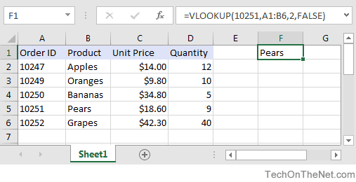
Make use of the VLOOKUP function to seek out a value in a table. Phrase structure VLOOKUP (lookup_value, table_array, col_index_num, [range_lookup] For instance: =VLOOKUP(A 2, A 10: C 20,2, REAL) =VLOOKUP("Fontana", B 2: E 7,2, FALSE) =VLOOKUP(A 2,'Customer Facts'! A: F,3, FALSE) Disagreement name Summary lookup_value (required) The value you intend to look up. The worth you want to look up should be in the initial column of the variety of cells you specify in the table_array disagreement.

Lookup_value can be a value or a recommendation to a cell. table_array (called for) The variety of cells in which the VLOOKUP will certainly look for the lookup_value and also the return value. You can utilize a called variety or a table, and you can utilize names in the debate as opposed to cell recommendations.

The cell range also needs to include the return worth you intend to find. Find out exactly how to choose varieties in a worksheet. col_index_num (required) The column number (starting with 1 for the left-most column of table_array) which contains the return value. range_lookup (optional) A rational value that specifies whether you want VLOOKUP to discover an approximate or a precise match: Approximate match - 1/TRUE assumes the initial column in the table is sorted either numerically or alphabetically, as well as will certainly after that search for the closest value.

For instance, =VLOOKUP(90, A 1: B 100,2, REAL). Precise match - 0/FALSE searches for the exact value in the initial column. For instance, =VLOOKUP("Smith", A 1: B 100,2, FALSE). There are 4 items of information that you will certainly need in order to build the VLOOKUP syntax: The worth you desire to seek out, also called the lookup worth.

The Facts About Excel Vlookup Function Revealed

Keep in mind that the lookup worth should constantly remain in the first column in the variety for VLOOKUP to function appropriately. For instance, if your lookup value remains in cell C 2 after that your range should begin with C. The column number in the range which contains the return worth. For instance, if you specify B 2:D 11 as the array, you ought to count B as the very first column, C as the 2nd, and more.

If you don't specify anything, the default value will certainly constantly hold true or approximate suit. Currently place every one of the above together as adheres to: =VLOOKUP(lookup value, variety consisting of the lookup worth, the column number in the array consisting of the return value, Approximate suit (REAL) or Precise suit (FALSE)). Right here are a few instances of VLOOKUP: Issue What failed Wrong worth returned If range_lookup is TRUE or overlooked, the initial column requires to be arranged alphabetically or numerically.

Either kind the very first column, or make use of FALSE for an exact match. #N/ A in cell If range_lookup is TRUE, then if the worth in the lookup_value is smaller sized than the smallest value in the very first column of the table_array, you'll obtain the #N/ An error value. If range_lookup is FALSE, the #N/ A mistake worth shows that the precise number isn't found.

#REF! in cell If col_index_num is above the variety of columns in table-array, you'll get the #REF! error worth. For more info on dealing with #REF! errors in VLOOKUP, see How to correct a #REF! mistake. #VALUE! in cell If the table_array is much less than 1, you'll get the #VALUE! error value.

#NAME? in cell The #NAME? error value usually means that the formula is missing out on quotes. To seek out an individual's name, ensure you use quotes around the name in the formula. For instance, enter the name as "Fontana" in =VLOOKUP("Fontana", B 2: E 7,2, FALSE). For even more details, see How to correct a #NAME! mistake.

Top Guidelines Of Vlookup Formula

Find out just how to make use of absolute cell referrals. Don't keep number or day values as text. When browsing number or day values, make certain the information in the very first column of table_array isn't stored as message worths. Otherwise, VLOOKUP might return a wrong or unforeseen worth. Arrange the initial column Type the very first column of the table_array prior to using VLOOKUP when range_lookup is TRUE.

An enigma matches any type of single personality. An asterisk matches any kind of series of personalities. If you wish to discover an actual inquiry mark or asterisk, kind a tilde (~) in front of the personality. For instance, =VLOOKUP("Fontan?", B 2: E 7,2, FALSE) will look for all circumstances of Fontana with a last letter that can differ.

When looking message values in the very first column, make certain the data in the very first column does not have leading areas, trailing areas, irregular usage of straight (' or") and also curly (' or ") quote marks, or nonprinting characters. In these cases, VLOOKUP might return an unforeseen worth.

You can always ask a specialist in the Excel User Voice. Quick Reference Card: VLOOKUP refresher Quick Referral Card: VLOOKUP fixing ideas You Tube: VLOOKUP videos from Excel community specialists Everything you require to learn about VLOOKUP Just how to deal with a #VALUE! mistake in the VLOOKUP feature Just how to remedy a #N/ A mistake in the VLOOKUP function Introduction of formulas in Excel Exactly how to prevent damaged solutions Identify mistakes in solutions Excel functions (indexed) Excel features (by category) VLOOKUP (cost-free preview).

To calculate delivery cost based upon weight, you can use the VLOOKUP function. In the instance shown, the formula in F 8 is: =VLOOKUP(F 7, B 6: C 10,2,1)* F 7 This formula makes use of the weight to find the right "price per kg" after that ... To override outcome from VLOOKUP, you can nest VLOOKUP in the IF feature.

vlookup in excel in 2 sheets vlookup in excel xls excel vba vlookup named range